Reproduction of Borjas & Breznau (2026),
“Ideological bias in the production of research findings”

Abstract

This report independently reproduces the main result of Borjas & Breznau (2026), a study of whether researchers' political ideology shapes the findings they produce. Using the Crowdsourced Replication Initiative, in which 71 teams estimated 1,253 models of the effect of immigration on support for social programs, the paper reports that pro-immigration teams estimate more positive effects and anti-immigration teams more negative ones. Reimplementing the authors' weighted, team-clustered regressions in R, I reproduce all nine columns of the paper's Table 1 exactly, including the headline Pro − Anti difference in the mean average marginal effect of 0.085 (SE 0.031, p = 0.008). Ten pre-specified robustness checks (alternative inference, controls, weighting, and sample restrictions) preserve the sign in every case and statistical significance in nine of ten; the sole exception is dropping all controls, which is consistent with the paper's own claim that discipline composition is the load-bearing control. The headline claim holds up, with the honest caveat that the association is modest in size and depends on conditioning on team composition.

1. What the main result is, and whether it reproduces

The headline claim is that team ideology predicts the estimated effect of immigration on support for social programs (the average marginal effect, AME): teams whose members are more pro-immigration produce more positive AMEs, and anti-immigration teams produce more negative ones. The paper's main quantitative result is Table 1: nine regressions of a model-level outcome on an ideology measure, with the “Pro − Anti” row giving the headline contrast.

I reproduced Table 1 exactly. The per-unit coefficient on the team mean immigration sentiment (column 1) is 0.0109 (SE 0.0057); across the full 1–6 scale this is 0.054 (0.029), matching the number stated in the paper's text. The central Pro − Anti difference (column 3) is 0.085 (0.031, p = 0.008): pro-immigration-majority teams estimate AMEs about 0.085 points higher than anti-immigration teams. Every coefficient, standard error, and R² in all nine columns matches the published table to the reported precision (≤ 0.001).

Table 1, reproduced vs. published

Column	Term	Published est. (SE)	Reproduced est. (SE)	Reproduced p	Match
(1) AME	Mean sentiment (proindex)	0.011 (0.006) *	0.0109 (0.0057)	0.061	yes
(2) AME	% anti-immigration (p12)	−0.050 (0.025) **	−0.0504 (0.0253)	0.050	yes
(2) AME	% pro-immigration (p56)	0.023 (0.019)	0.0235 (0.0193)	0.229	yes
(2) AME	Pro − Anti (p56 − p12)	0.074 (0.024) **	0.0739 (0.0243)	0.003	yes
(3) AME	Anti team (group1)	−0.057 (0.031) *	−0.0572 (0.0306)	0.066	yes
(3) AME	Pro team (group3)	0.027 (0.015) *	0.0273 (0.0147)	0.069	yes
(3) AME	Pro − Anti (group3 − group1)	0.085 (0.031) **	0.0845 (0.0310)	0.008	yes
(4) extreme neg.	Mean sentiment (proindex)	−0.051 (0.021) **	−0.0514 (0.0207)	0.015	yes
(5) extreme neg.	% anti-immigration (p12)	0.081 (0.103)	0.0809 (0.1028)	0.434	yes
(5) extreme neg.	% pro-immigration (p56)	−0.161 (0.064) **	−0.1607 (0.0643)	0.015	yes
(5) extreme neg.	Pro − Anti (p56 − p12)	−0.242 (0.107) *	−0.2416 (0.1074)	0.028	yes
(6) extreme neg.	Anti team (group1)	0.150 (0.123)	0.1500 (0.1232)	0.227	yes
(6) extreme neg.	Pro team (group3)	−0.124 (0.044) **	−0.1239 (0.0440)	0.006	yes
(6) extreme neg.	Pro − Anti (group3 − group1)	−0.274 (0.125) *	−0.2739 (0.1252)	0.032	yes
(7) extreme pos.	Mean sentiment (proindex)	0.019 (0.012) *	0.0192 (0.0115)	0.099	yes
(8) extreme pos.	% anti-immigration (p12)	−0.130 (0.057) *	−0.1304 (0.0569)	0.025	yes
(8) extreme pos.	% pro-immigration (p56)	−0.016 (0.041)	−0.0161 (0.0413)	0.697	yes
(8) extreme pos.	Pro − Anti (p56 − p12)	0.114 (0.045) *	0.1142 (0.0458)	0.015	yes
(9) extreme pos.	Anti team (group1)	−0.070 (0.037) *	−0.0695 (0.0378)	0.070	yes
(9) extreme pos.	Pro team (group3)	0.017 (0.034)	0.0173 (0.0340)	0.612	yes
(9) extreme pos.	Pro − Anti (group3 − group1)	0.087 (0.035) *	0.0868 (0.0347)	0.015	yes

R² reproduced (published): (1) 0.062 (0.062), (2) 0.065 (0.065), (3) 0.071 (0.071), (4) 0.096 (0.096), (5) 0.115 (0.115), (6) 0.133 (0.133), (7) 0.087 (0.087), (8) 0.090 (0.090), (9) 0.089 (0.089).

All regressions: N = 1,253 model-level observations from 71 teams; dependent variable is the AME (cols 1–3) or a binary indicator for an extreme-and-significant AME in the negative (cols 4–6) or positive (cols 7–9) tail; controls are standardized statistical skill, standardized topic experience, team-size fixed effects, and discipline-composition fixed effects; weighted by 1/(number of models per team); team-clustered robust standard errors.

Sources for each published number

Published number	Source
Table 1 coefficients, SEs, significance markers, R²	Open-access full text of the paper, Table 1, Europe PMC PMC12757037 (opened in this session; the paywalled publisher page returned HTTP 403)
“0.054 (0.029)” full-range sentiment effect	Paper text, same source (the abstract and Table 1 caption also come from here)
Cross-check of all Table 1 numbers	code/Log Files/02_Main_Regs.log in this folder (the Stata output the README names as the result file for Table 1)
Estimator definition (weights, controls, clusters, tail cutoffs)	code/Stata Main Results/02_Main_Regs.do and code/Stata Main Results/01_Data_Prep.do in this folder
Analysis data	data/df.dta in this folder (designated as the analysis file by README.md)

I did not rely on memory for any published number.

2. Analysis decisions the paper did not settle for me

1. Starting point. I begin from data/df.dta, the prepared analysis file, rather than re-running the Stata preparation from cri.csv. This takes the authors' recodes and hot-deck imputations (notably for team 27) as given and matches the file the README designates as the analysis data.
2. Reproduction toolchain. No Stata is installed, so I reimplemented reg ..., [aw=1/nmodel] cluster(teamid) in R as weighted lm() plus a cluster-robust HC1 covariance (sandwich::vcovCL). I verified that HC1 — not HC0 or CR2 — reproduces Stata's standard errors to six decimals on the baseline model before running the rest.
3. Discipline fixed-effect base category. i.mdegree uses the lowest discipline code (0) as reference. This choice does not affect the reported ideology contrasts but does change the meaning of the discipline coefficients (not reported here).
4. Rows with missing AME. One of 1,254 rows has a missing AME and is dropped, matching Stata's drop if ame==. and giving the published N = 1,253.
5. Definition of the “extreme” tails. The paper text describes the tail outcomes as “<10th percentile and P < 0.05”, but the code hard-codes fixed AME cutoffs (AME > 0.052 or AME < −0.071) together with |z| > 1.645, and the outcomes are pre-built in df.dta. I used those built-in neg10s/pos10s indicators and did not recompute percentiles.
6. Weights for the binary outcomes. The Stata code uses importance weights ([iw=1/nmodel]) for the tail models and analytic weights ([aw=1/nmodel]) for the AME models. For WLS point estimates and the HC1 covariance these are identical, so I used the same weighting throughout.
7. Inference. I use team-clustered robust SEs with t critical values and degrees of freedom = number of teams − 1 = 70, matching Stata. I add no further finite-sample correction.
8. Full-scale interpretation of the continuous measure. The paper reports the per-unit coefficient in Table 1 but discusses a 1-to-6 move (×5) in the text. I report both.
9. Significance markers. For the four tail-model “Pro − Anti” differences (columns 5, 6, 8, 9) the paper prints a single *, although the reproduced two-sided p-values (0.028, 0.032, 0.015, 0.015) fall below 0.05 and the paper's own caption defines ** as P < 0.05. I report my p-values and flag the discrepancy rather than copying the stars.

I also checked the paper's claim that the weighted model-level regression is numerically identical to a team-level regression. It is, to all displayed digits, so I do not treat team-level aggregation as a separate robustness check.

3. Robustness

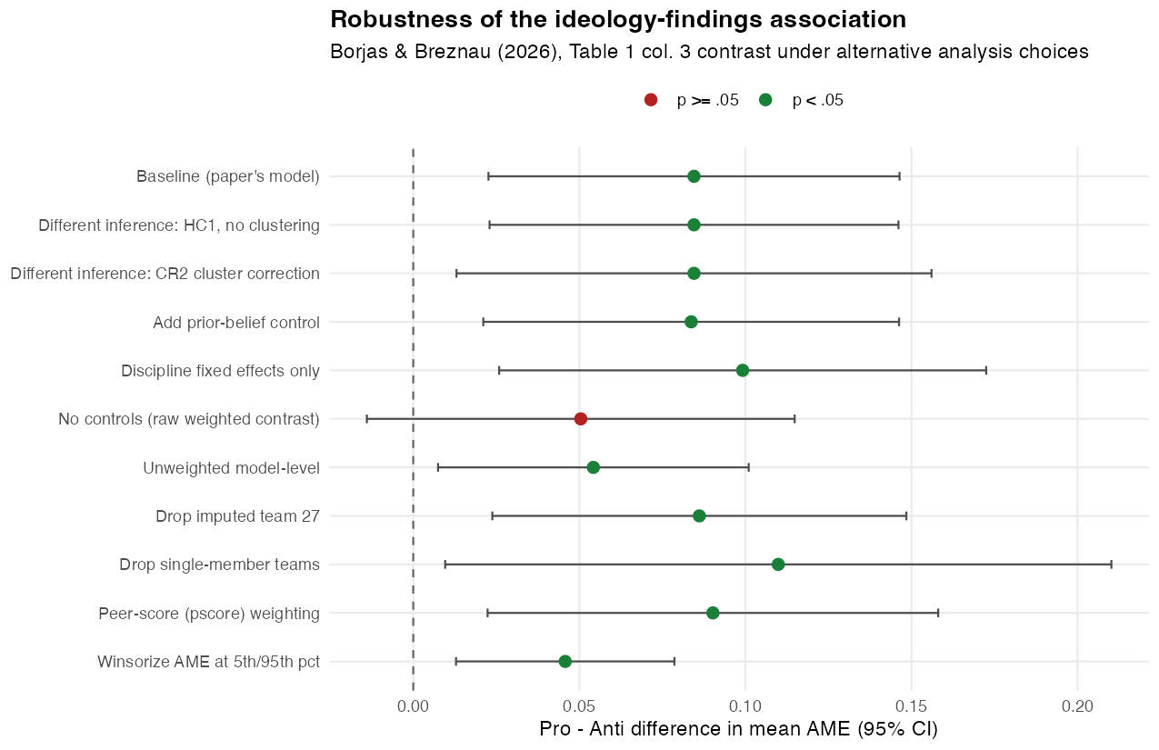
I fixed the research question (“does team ideology predict the estimated AME?”) and the headline estimand (the Pro − Anti difference in mean AME, Table 1 column 3), then varied the analysis choices. Before running anything I listed ten defensible alternatives and recorded which I expected to change the conclusion:

#	Alternative choice	Rationale	Expected to change conclusion?
1	HC1 heteroskedasticity-robust, no clustering	Tests whether team clustering drives inference	No
2	CR2 small-sample cluster correction	71 clusters is comfortably large, but CR2 is the conservative choice	Possibly (slightly wider CI)
3	Add prior-belief control	Belief in the hypothesis as an alternative explanation	No
4	Discipline fixed effects only	Paper argues discipline composition is the load-bearing control	No (possibly stronger)
5	No controls at all	Tests whether the result survives a raw contrast	Yes
6	Unweighted model-level	Gives teams with many models more weight	Possibly (magnitude shifts)
7	Drop imputed team 27	Removes the only hot-deck-imputed team	No
8	Drop single-member teams	Solo researchers' ideology is measured differently	No (wider CI)
9	Peer-score (pscore) weighting	Addresses publication/selection bias, as in the paper's supplements	No
10	Winsorize AME at the 5th/95th percentiles	Robustness to extreme estimates	Possibly (attenuated)

Results

Specification	Pro − Anti est.	SE	p	95% CI	Sig.
Baseline (paper's model)	0.0845	0.0310	0.008	[0.023, 0.146]	**
1. HC1, no clustering	0.0845	0.0314	0.007	[0.023, 0.146]	**
2. CR2 cluster correction	0.0845	0.0359	0.021	[0.013, 0.156]	**
3. Add prior-belief control	0.0837	0.0314	0.010	[0.021, 0.146]	**
4. Discipline fixed effects only	0.0992	0.0368	0.009	[0.026, 0.173]	**
5. No controls (raw contrast)	0.0504	0.0323	0.123	[−0.014, 0.115]	n.s.
6. Unweighted model-level	0.0542	0.0234	0.024	[0.007, 0.101]	**
7. Drop imputed team 27	0.0861	0.0312	0.007	[0.024, 0.149]	**
8. Drop single-member teams	0.1099	0.0500	0.032	[0.010, 0.210]	**
9. Peer-score (pscore) weighting	0.0902	0.0340	0.010	[0.022, 0.158]	**
10. Winsorize AME at 5th/95th pct	0.0458	0.0165	0.007	[0.013, 0.079]	**

** p < 0.05; n.s. p ≥ 0.05.

The sign of the Pro − Anti difference is positive in every specification. Nine of the ten alternatives remain significant at the 5% level and the point estimates stay in a narrow band (0.046 to 0.110). The only specification that loses significance is dropping all controls (0.050, p = 0.12): without conditioning on team composition the contrast shrinks by about 40%. Notably, keeping only the discipline fixed effects makes the estimate stronger (0.099), so the sensitivity is not to “too many controls” generally but to whether discipline composition is held constant. This is consistent with the paper's own statement that the discipline vector is the key control. Winsorizing the AME (which removes the tail observations the paper separately models) roughly halves the estimate but keeps it significant, as expected.

4. Verdict