Topic 11 Meta-analyses - a very brief introduction
Quantitative research tends to ask to broad questions: (1) does a certain effect exist? (2) when and where is it stronger or weaker? Neither of them can be answered by a single study, which will always take place in a specific context and yield probabilistic results. Therefore, quantitative research needs to be synthesized. Statistical meta-analyses are one way to take the results of many studies that consider the same phenomenon to test whether there is a significant effect overall, what its size is likely to be, and whether its size is moderated by methodological or substantive variables.
Meta-analyses work best (or, at least, are most straight-forward) when there is a large body of research that tested a specific phenomenon. One interesting case study was the ManyLabs2 project that attempted to replicate many classic findings in the behavioural sciences. They ran a set of studies with about 65 samples for each, drawn from all continents, which once again showed that many classic studies do not replicate, but also that there are some interesting contextual differences.
Below, I show how to analyse their replication data for one of the most famous papers in behavioural economics, which has accumulated more than 20,000 citations. This is not a complete guide to running meta-analyses - those are linked to in further resources at the bottom. Instead, it is meant to give you a first taste of why you might want to run them and how to approach it in R.
11.1 A famous finding to be replicated
Back in 1981, Tversky and Kahneman provided evidence that people’s decision making systematically differs from what we might expect under a rational-choice model. In the study considered here, they asked people to imagine that they were in a store, shopping for a jacket and a calculator. In each condition, one of the items was described as expensive (125 USD), and one as cheap (15 USD). Then, the participants were told that either the expensive or the cheap item was available with a 5 USD discount at another branch 20 minutes away. Rationally, we might expect that it does not matter which of the two items we could save 5 USD on, yet participants in the original study were much more likely to say that they were willing to make the trip when the cheap item was on sale (68%) than when the expensive item was on sale (29%). Their result was highly significant, p < .0001, OR = 4.96, 95% CI = [2.55, 9.90]).
11.2 The replications
ManyLabs2 ran 57 replications of this survey experiment. Their results were not particularly consistent - one showed an effect in the opposite direction, 34 did not find a significant effect, and just 23 replicated the original paper with a significant finding. However, it needs to be noted that these replications were not designed to be considered on their own - individually, they are severely underpowered, with a median sample size of 96. Therefore, we need to aggregate them.
You can download their data here (pre-processed) if you want to run the analyses yourself, or even get the full ManyLabs2 dataset if you want to try this for a different study..
pacman::p_load(tidyverse, magrittr)
ML2_framing <- read_rds("files/ML2_framing.RDS")
get_OR <- function(tb, ci = .95,
                   success = "yes", failure = "no",
                   group1 = "cheaper", group2 = "expensive") {

  OR <- (tb[group1, success]/tb[group1,failure])/(tb[group2,success]/tb[group2,failure])

  ci_lower <- exp(log(OR) - qnorm(1-(1-ci)/2)*sqrt(sum(1/tb)))
  ci_upper <- exp(log(OR) + qnorm(1-(1-ci)/2)*sqrt(sum(1/tb)))

  p <- tb %>% chisq.test() %>% .$p.value

  tibble(OR = OR, ci_lower = ci_lower, ci_upper = ci_upper, N = sum(tb), p_value = p)

}

OR <- ML2_framing %>%
  split(.$Lab) %>%
  map_dfr(~ .x %$% table(condition, response) %>% get_OR(), .id = "Lab")
## Warning in chisq.test(.): Chi-squared approximation may be incorrect
## Warning in chisq.test(.): Chi-squared approximation may be incorrecttable(right_direction = OR$OR>1, significant = OR$p_value < .05)
range(OR$OR)
#Add Weird variable back into that summary
weirdness <- ML2_framing %>% select(Lab, Weird) %>% distinct()
OR <- OR %>% left_join(weirdness)## Joining, by = "Lab"## significant
## right_direction FALSE TRUE
## FALSE 1 0
## TRUE 33 23
## [1] 0.5926724 5.444444411.3 Meta-analysis across the replications
Running a meta-analysis across the replication results allows us to test whether we have evidence of a significant effect overall, to estimate the effect size with greater precision, and to test whether the effect size is moderated (i.e. changed) by any variables. Here, I will test for moderation by the WEIRDness of the sample, i.e. whether it is located in a Western country2 Given that the finding originated among US University students, this is an important question.
All that we need for a meta-analysis is an effect size per study alongside a measure of its precision (usually either a standard error or a confidence interval). Meta-analyses can be run based on any effect size measure - in this case, Odds Ratios. However, they need to be entered in a way that is linear, i.e. where each step-change corresponds to the same change in effect. With Odds Ratios, that is not the case - from 0.5 to 1, the odds double, while the change from 1 to 1.5 is smaller. Therefore, meta-analyses are run on log-odds. If we had a mean difference, such as Cohen’s d, we could enter it straight-away.
I will use the metagen() function from the meta package to show you how quick it can be to run a meta-analysis. It is probably the most versatile function for meta-analyses, and can be tuned with a lot of different parameters. Therefore, this is one of the few instances when I would not recommend that you start by reading ?metagen - if you want to explore the function further, rather have a look at the Doing Meta-Analysis in R online book.
The results of the meta-analysis will be shown in a forest plot here. Each line describes on of the studies (or here, the results from one lab) - you might note how sample size relates to the width of the confidence interval, and what sample sizes are associated with the most extreme estimates. I show both the results of a fixed-effects and a random-effects meta-analysis. A fixed-effects meta-analysis is straight-forward: it calculates the average of the effect sizes, inversely weighted by their variance, so that more precise estimates gain greater weight. However, this is only appropriate if we believe that all studies come from a single homogeneous population, which is hardly ever the case. Usually, we therefore focus on random-effects models, which assumes that our studies are sampling different populations. Therefore, we no longer just estimate the weighted mean effect size, but also the variance of the effect sizes, which is denoted as τ2. Here, the two models yield very similar results.3
pacman::p_load(tidyverse, meta)

#See hidden code above if you want to see how I calculated the effect size per sample based on the full ManyLabs2 dataset.
#When doing a meta-analysis on published papers, you might just collect this kind of information from each paper in a spreadsheet
head(OR)
## # A tibble: 6 x 7
## Lab OR ci_lower ci_upper N p_value Weird
## <chr> <dbl> <dbl> <dbl> <int> <dbl> <int>
## 1 Australia1 1.88 0.792 4.46 97 0.222 1
## 2 Australia2 1.55 0.767 3.13 137 0.295 1
## 3 Austria1 2.00 0.894 4.49 102 0.135 1
## 4 Belgium1 1.51 0.684 3.33 100 0.413 1
## 5 Canada1 3.5 1.59 7.68 121 0.00271 1
## 6 Chile1 0.593 0.233 1.51 81 0.387 1#Convert to log-odds and calculate standard error
log_OR <- OR %>% mutate(across(c(OR, ci_lower, ci_upper), log), se = (ci_upper - ci_lower)/(2*qnorm(.975)))
#Run meta-analysis
meta_analysis <- metagen(OR, se, studlab = Lab, data = log_OR, byvar = Weird,
sm = "OR", method.tau = "SJ", n.e = N)
#Create forest plot that summarises results
forest(meta_analysis, sortvar = -TE, text.fixed = "Fixed effects: overall estimate",
text.random = "Random effects: overall estimate", leftcols = c("studlab", "n.e"), leftlabs = c("Lab", "N"))## Warning: Use argument 'subgroup' instead of 'byvar' (deprecated).## png
## 2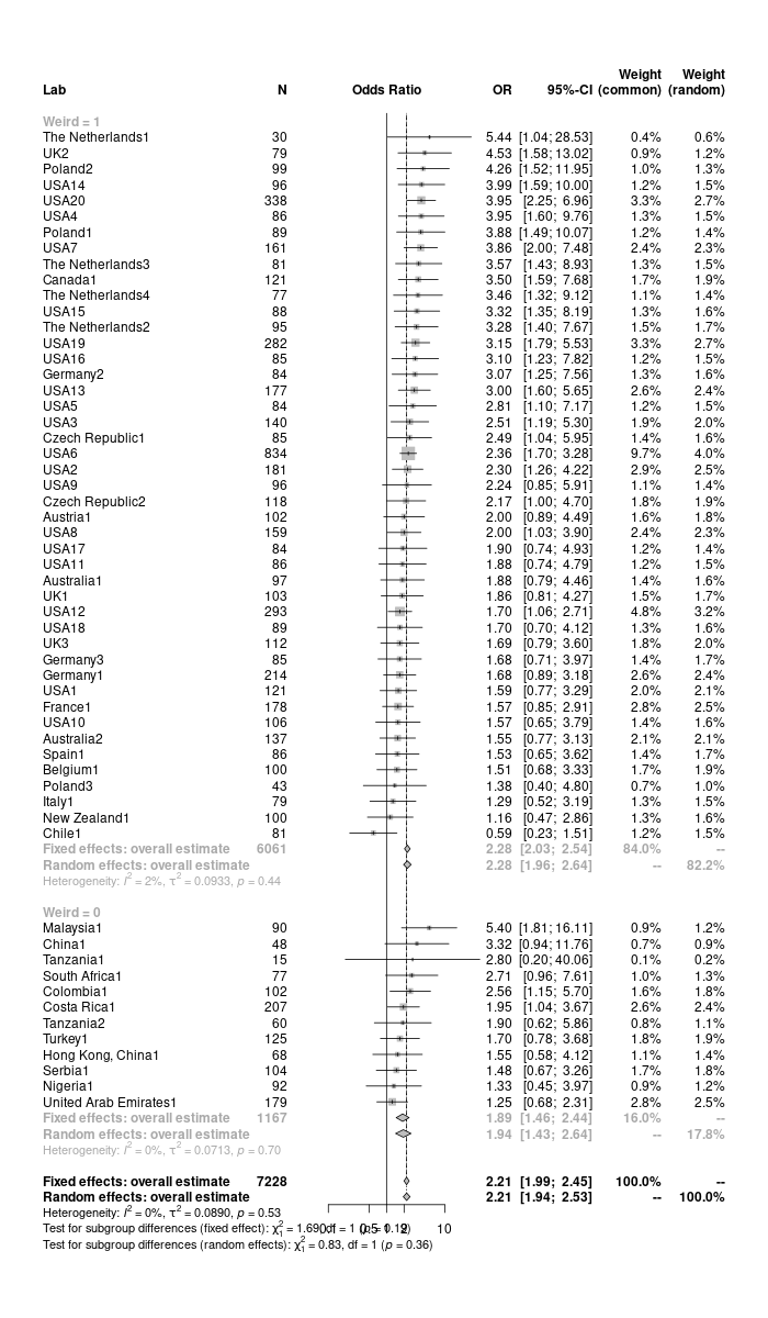
Figure 11.1: Forest plot for meta-analysis
From the meta-analysis, we can conclude that ManyLabs2 provided strong evidence for the framing effect established by Tversky & Kahneman (1981). However, you should note that the effect size is much smaller than what they found (even below their confidence interval), and that there is a trend that the effect might be weaker in non-WEIRD samples (note that metagen also offers a significance test for this in the full output).
## Number of studies combined: k = 57
## Number of observations: o = 7228
##
##                          OR           95%-CI     z  p-value
## Common effect model  2.2088 [1.9935; 2.4473] 15.15 < 0.0001
## Random effects model 2.2141 [1.9366; 2.5314] 11.63 < 0.0001
##
## Quantifying heterogeneity:
##  tau^2 = 0.0890 [0.0000; 0.0781]; tau = 0.2983 [0.0000; 0.2796]
##  I^2 = 0.0% [0.0%; 31.2%]; H = 1.00 [1.00; 1.21]
##
## Test of heterogeneity:
##      Q d.f. p-value
##  54.60   56  0.5279
##
## Results for subgroups (common effect model):
##             k     OR           95%-CI     Q  I^2
## Weird = 1  45 2.2752 [2.0344; 2.5446] 44.76 1.7%
## Weird = 0  12 1.8904 [1.4630; 2.4428]  8.16 0.0%
##
## Test for subgroup differences (common effect model):
##                    Q d.f. p-value
## Between groups  1.69    1  0.1942
## Within groups  52.92   55  0.5547
##
## Results for subgroups (random effects model):
##             k     OR           95%-CI  tau^2    tau
## Weird = 1  45 2.2758 [1.9607; 2.6415] 0.0933 0.3055
## Weird = 0  12 1.9417 [1.4286; 2.6392] 0.0713 0.2670
##
## Test for subgroup differences (random effects model):
##                     Q d.f. p-value
## Between groups   0.83    1  0.3618
##
## Details on meta-analytical method:
## - Inverse variance method
## - Sidik-Jonkman estimator for tau^2
## - Q-profile method for confidence interval of tau^2 and tau
11.4 Further resources
- This guide to running meta-analyses in R starts from the basics but then quite quickly reaches the level of detail needed to actually produce trustworthy results.
- This collaborative “syllabus” has a wealth of material that addresses both theoretical concerns and practical know-how.
WEIRD refers to Western, Educated, Industrialized, Rich, and Democratic. The acronym was coined by Henrich, Heine, and Norenzayan (2010) in a scathing critique of the over-reliance on behavioural scientists on such samples while claiming to study universal human traits. This has been debated much over the past decade - the jury is still out on whether things have improved.↩︎
Random-effects model have become the standard, at least in psychology. However, they give comparatively greater weight to smaller studies, as you might notice in the forest plot. Given that small studies might be the most biased - particularly when there is publication bias, so that underpowered studies can only get published with exaggerated effects, some have argued that the default should be to run fixed-effects models. You can find a slightly longer discussion and references here↩︎