This package aims to speed up research projects in social psychology (and related fields). For that, it primarily includes some functions that help lay the groundwork and others that facilitate the reporting of results.

Among others, the package can help with the following:

Creating scales, including reverse-coding and reporting their internal consistency,
Creating correlation tables in APA style, including descriptive statistics and confidence intervals, and an option to use survey weights, multiple imputation or full-information maximum-likelihood estimation
Creating regression tables comparing standardised and non-standardised regression coefficients, and comparing the F-change between two nested models
Formatting numbers for statistical reporting, including rounding with trailing zeros, or displaying numbers as p-values or as confidence intervals
Data entry and transfer, for quick interactive use. This includes splitting clipboard content into vectors, converting tibbles to tribble code, or obtaining nicely formatted code and results to paste into another application

Why use this package?

There are many packages that support data analysis and reporting. For instance, the psych package offers functions to create scales, while the modelsummary package offers options to create customisable tables in a wide variety of output format. They power many of the functions offered here ‘under the hood.’

apa and papaja are two packages that directly support the reporting of results in APA style - they can complement this package well. However, none of the existing offered quite what we needed. This package

takes an end-to-end view of the data analysis process, streamlining time-consuming steps at various stages
offers analysis templates that make it easy to get started, particularly for R novices,
prioritises publication-readiness and good reporting practices over customisability in creating tables and charts
integrates with the tidyverse by supporting tidy evaluation and returning tibbles where possible

Installation

You can install timesaveR from GitHub with the command below. If you do not have the remotes-package installed, run install.packages("remote") first.

remotes::install_github('lukaswallrich/timesaveR')

Get started

There are many functions in the package, and we will create vignettes detailing various use cases. However, the following can give you an initial flavor. The examples use data from the European Social Survey Wave 7 (2014). Here, I ignore survey weights. However, the package offers similar functions for analysing weighted survey data, which are explained in the survey data vignette.

Load the package

(I also load dplyr since that is the recommended usage - of course, there are base R alternatives for all of the steps.)

library(dplyr)
#> 
#> Attaching package: 'dplyr'
#> The following objects are masked from 'package:stats':
#> 
#>     filter, lag
#> The following objects are masked from 'package:base':
#> 
#>     intersect, setdiff, setequal, union
library(timesaveR)
#> Note re timesaveR: Many functions in this package are alpha-versions - please treat results with care and report bugs and desired features.

Create scales

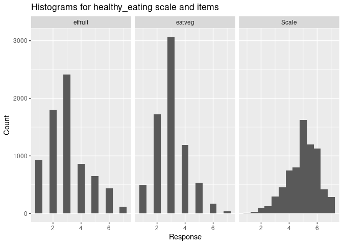
Let’s create scales for health behaviours and depressive symptoms, each including some reverse coding.

scales <- list(
  depression = c("fltdpr", "flteeff", "slprl", "wrhpp", "fltlnl", 
                 "enjlf", "fltsd", "cldgng"),
  healthy_eating = c("etfruit", "eatveg")
  )
  
scales_reverse <- list(
  depression = c("wrhpp", "enjlf"),
  healthy_eating = c("etfruit", "eatveg")
)

scales <- make_scales(ess_health, items = scales, reversed = scales_reverse)
#> The following scales will be calculated with specified reverse coding: depression, healthy_eating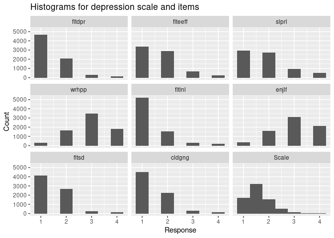


#Check descriptives, including reliability
scales$descriptives
#> # A tibble: 2 × 10
#>   Scale      n_items reliability reliability_method  mean    SD reversed rev_min
#>   <chr>        <int>       <dbl> <chr>              <dbl> <dbl> <chr>      <dbl>
#> 1 depression       8       0.802 cronbachs_alpha     1.67 0.484 wrhpp e…       1
#> 2 healthy_e…       2       0.658 spearman_brown      4.97 1.11  etfruit…       1
#> # ℹ 2 more variables: rev_max <dbl>, text <chr>

#Add scale scores to dataset
ess_health <- bind_cols(ess_health, scales$scores)

Report correlations and descriptive statistics

Next, we are often interested in descriptive statistics, variable distributions and correlations.

ess_health %>% select(agea, health, depression, healthy_eating) %>% 
    cor_matrix() %>% report_cor_table()

Variable	M (SD)	1	2	3
agea	50.61 (18.51)
health	2.26 (0.92)	.28 *** [0.25, 0.30]
depression	1.67 (0.48)	.03 * [0.00, 0.05]	.42 *** [0.40, 0.44]
healthy_eating	4.97 (1.11)	.17 *** [0.15, 0.19]	-.09 *** [-0.11, -0.07]	-.13 *** [-0.15, -0.10]
M and SD are used to represent mean and standard deviation, respectively. Values in square brackets indicate the 95% confidence interval for each correlation.
† p < .1, * p < .05, p < .01, * p < .001


#It is often helpful to rename variables in this step
#Use get_rename_tribbles(ess_health) to get most of this code
var_renames <- tibble::tribble(
    ~old,     ~new,     
    "agea",   "Age",  
    "health",  "Poor health",
    "depression",  "Depression",
    "healthy_eating",  "Healthy eating",
)

#A rename tibble or vector automatically only selects the variables included into it
ess_health %>% cor_matrix(var_names = var_renames) %>% report_cor_table()

Variable	M (SD)	1	2	3
Age	50.61 (18.51)
Poor health	2.26 (0.92)	.28 *** [0.25, 0.30]
Depression	1.67 (0.48)	.03 * [0.00, 0.05]	.42 *** [0.40, 0.44]
Healthy eating	4.97 (1.11)	.17 *** [0.15, 0.19]	-.09 *** [-0.11, -0.07]	-.13 *** [-0.15, -0.10]
M and SD are used to represent mean and standard deviation, respectively. Values in square brackets indicate the 95% confidence interval for each correlation.
† p < .1, * p < .05, p < .01, * p < .001


#Often, it is also interesting to include variable distributions
ess_health %>% cor_matrix(var_names = var_renames) %>%
    report_cor_table(add_distributions = TRUE, data = ess_health)

Variable	M (SD)	1	2	3
Age	50.61 (18.51)
Poor health	2.26 (0.92)	.28 *** [0.25, 0.30]
Depression	1.67 (0.48)	.03 * [0.00, 0.05]	.42 *** [0.40, 0.44]
Healthy eating	4.97 (1.11)	.17 *** [0.15, 0.19]	-.09 *** [-0.11, -0.07]	-.13 *** [-0.15, -0.10]
M and SD are used to represent mean and standard deviation, respectively. Values in square brackets indicate the 95% confidence interval for each correlation.
† p < .1, * p < .05, p < .01, * p < .001

Describe categorical variables and their relation with an outcome

Often, we are also interested in how the means of an outcome variable differ between different groups. It can be fiddly to get these tables and the pairwise significance tests done, but this function does it in a breeze.

# Start with this in the console - that gets you 80% of the tribbles below.
# get_rename_tribbles(ess_health, gndr, cntry)

var_renames <- tribble(
    ~old,     ~new,     
    "gndr",   "Gender",  
    "cntry",  "Country"
)

level_renames <- tribble(
    ~var,     ~level_old, ~level_new, 
    "gndr",   "1",        "male",       
    "gndr",   "2",        "female",       
    "cntry",  "DE",       "Germany",      
    "cntry",  "FR",       "France",      
    "cntry",  "GB",       "UK"
)

report_cat_vars(ess_health, health, gndr, cntry, var_names = var_renames, 
              level_names = level_renames)

	N	Share	M (SD)
Gender
male	3482	48.2%	2.23 (0.90) ^a
female	3744	51.8%	2.30 (0.93) ^b
Country
Germany	3045	42.1%	2.34 (0.88) ^a
France	1917	26.5%	2.29 (0.89) ^a
UK	2264	31.3%	2.14 (0.97) ^b
M and SD are used to represent mean and standard deviation for health for that group, respectively.
Within each variable, the means of groups with different superscripts differ with p < .05 (p-values were adjusted using the Holm-method.)

Report regression models with standardized coefficients

In psychology, it is often expected that regression models are reported with both unstandardised (B) and standardized (beta) coefficients. This can be fiddly as separate tables will contain too much redundant information. The functions below easily run a model with standardised variables and create a publication-ready table.

ess_health$gndr <- factor(ess_health$gndr)

#Standard lm model
mod1 <- lm(depression ~ agea + gndr + health + cntry, ess_health)

#Model with standardised coefficients

mod2 <- lm_std(depression ~ agea + gndr + health + cntry, ess_health)

report_lm_with_std(mod1, mod2)

	B (SE)	β [95% CI]
(Intercept)	1.20 (0.02)***	-0.14 [-0.18, -0.10]
agea	-0.00 (0.00)***	-0.10 [-0.12, -0.08]
gndr2	0.12 (0.01)***	0.24 [0.20, 0.28]
health	0.23 (0.01)***	0.44 [0.42, 0.47]
cntryFR	-0.01 (0.01)	-0.02 [-0.08, 0.03]
cntryGB	0.04 (0.01)**	0.08 [0.03, 0.13]
N	7171
R²	.20
F-tests	F(5, 7165) = 358.25, p < .001
Given that dummy variables lose their interpretability when standardized (Fox, 2015), β for dummy variables are semi-standardized, indicating the impact of that dummy on the standardized outcome variable.
† p < .1, * p < .05, p < .01, * p < .001


#Often the coefficients should be renamed - get_coef_rename_tribble(mod1) 
#is the starting point. In that, markdown formatting can be used.

coef_names <- tribble(
  ~old,           ~new,           
   "(Intercept)",  "*(Intercept)*", 
   "agea",         "Age",        
   "gndr2",        "Gender *(female)*",       
   "health",       "Poor health",      
   "cntryFR",      "France *(vs DE)*",     
   "cntryGB",      "UK *(vs DE)*"
)

report_lm_with_std(mod1, mod2, coef_renames = coef_names)

	B (SE)	β [95% CI]
(Intercept)	1.20 (0.02)***	-0.14 [-0.18, -0.10]
Age	-0.00 (0.00)***	-0.10 [-0.12, -0.08]
Gender (female)	0.12 (0.01)***	0.24 [0.20, 0.28]
Poor health	0.23 (0.01)***	0.44 [0.42, 0.47]
France (vs DE)	-0.01 (0.01)	-0.02 [-0.08, 0.03]
UK (vs DE)	0.04 (0.01)**	0.08 [0.03, 0.13]
N	7171
R²	.20
F-tests	F(5, 7165) = 358.25, p < .001
Given that dummy variables lose their interpretability when standardized (Fox, 2015), β for dummy variables are semi-standardized, indicating the impact of that dummy on the standardized outcome variable.
† p < .1, * p < .05, p < .01, * p < .001


#You can also easily display multiple nested models side-by-side and get the
#F-change significance test. For that, all models need to be fit on the same
#dataset, so that I will drop all missing data.

mod1 <- lm(depression ~ agea + gndr + health + cntry, tidyr::drop_na(ess_health))
mod2 <- lm_std(depression ~ agea + gndr + health + cntry, tidyr::drop_na(ess_health))


mod3 <- lm(depression ~ agea * gndr + eisced + health + cntry, tidyr::drop_na(ess_health))
mod4 <- lm_std(depression ~ agea * gndr + eisced + health + cntry, tidyr::drop_na(ess_health))

coef_names <- tribble(
  ~old,           ~new,           
   "(Intercept)",  "*(Intercept)*", 
   "agea",         "Age",        
   "gndr2",        "Gender *(female)*",       
   "health",       "Poor health",      
   "cntryFR",      "France *(vs DE)*",     
   "cntryGB",      "UK *(vs DE)*",
   "eisced",       "Education",
   "agea:gndr2",   "Age x Female",
)

report_lm_with_std(mod = list(mod1, mod3), mod_std = list(mod2, mod4),
                   coef_renames = coef_names, R2_change = TRUE)
#> Warning: Automatic coercion from double to character was deprecated in purrr 1.0.0.
#> ℹ Please use an explicit call to `as.character()` within `map_chr()` instead.
#> ℹ The deprecated feature was likely used in the timesaveR package.
#>   Please report the issue at
#>   <https://github.com/LukasWallrich/timesaveR/issues>.
#> This warning is displayed once every 8 hours.
#> Call `lifecycle::last_lifecycle_warnings()` to see where this warning was
#> generated.

	Model 1		Model 2
	B (SE)	β [95% CI]	B (SE)	β [95% CI]
(Intercept)	1.21 (0.02)***	-0.14 [-0.18, -0.10]	1.27 (0.02)***	-0.14 [-0.18, -0.10]
Age	-0.00 (0.00)***	-0.10 [-0.12, -0.08]	-0.00 (0.00)***	-0.14 [-0.17, -0.10]
Gender (female)	0.11 (0.01)***	0.24 [0.20, 0.28]	0.03 (0.03)	0.24 [0.20, 0.28]
Poor health	0.23 (0.01)***	0.44 [0.42, 0.46]	0.23 (0.01)***	0.44 [0.42, 0.46]
France (vs DE)	-0.01 (0.01)	-0.03 [-0.08, 0.02]	-0.01 (0.01)	-0.03 [-0.08, 0.02]
UK (vs DE)	0.04 (0.01)**	0.08 [0.03, 0.13]	0.04 (0.01)**	0.08 [0.03, 0.13]
Education			-0.00 (0.00)†	-0.02 [-0.04, 0.00]
Age x Female			0.00 (0.00)**	0.07 [0.02, 0.11]
N	6852		6852
R²	.20		.20
F-tests	F(5, 6846) = 337.06, p < .001		F(7, 6844) = 243.10, p < .001
Change	ΔR² = .00, F(2, 6844) = 6.78, p = .001
Given that dummy variables lose their interpretability when standardized (Fox, 2015), β for dummy variables are semi-standardized, indicating the impact of that dummy on the standardized outcome variable.
† p < .1, * p < .05, p < .01, * p < .001

Related/alternative packages

modelsummary allows you to create highly customisable tables with data summaries or the output of statistical models that can be saved in a wide range of formats.
apa mostly offers functions that turn the output of statistical tests (e.g., t-tests) into text, in line with APA guidelines.
papaja offers the opportunity to create full APA-style journal manuscripts in R. It’s apa_table function is a generic alternative to the table functions in this package, which support many more types of models, but includes fewer details.

timesaveR

Why use this package?

Installation

Get started

Load the package

Create scales

Report correlations and descriptive statistics

Describe categorical variables and their relation with an outcome

Report regression models with standardized coefficients

Related/alternative packages

Links

License

Citation

Developers

Dev status