Using survey weights
Large-scale social surveys often do not aim to recruit random samples, but rather oversample small groups that are of interest for sub-group analyses (e.g., ethnic minorities). In addition, they never quite succeed in recruiting representative samples. To ensure that the results of statistical models approximate population parameters, survey weights need to be used to give each participant a specific weight in analyses. You can find out more in this brief YouTube video or explore the more extensive guide to weights in the European Social Survey as an example.
Survey weights in timesaveR
Many functions in the timesaveR package have
alternatives that accept survey objects instead of dataframes. These
functions are designated by the svy_ prefix. The
svy_ functions ensure that all calculations (means,
correlations, tests) account for survey weights, providing accurate
population estimates rather than sample statistics. To use them, you
will first need to use the srvyr package to create a survey
object based on the dataframe.
Below, I show some analyses of the European Social Survey 2014 data using the correct survey weights.
Create scales
Let’s create scales for health behaviours and depressive symptoms,
each including some reverse coding. For that, we need to pass the survey
items (as well as any to be reversed) to the
svy_make_scale() function
  depression_items = c("fltdpr", "flteeff", "slprl", "wrhpp", "fltlnl",
                 "enjlf", "fltsd", "cldgng")

  healthy_eating_items = c("etfruit", "eatveg")

  depression_reversed = c("wrhpp", "enjlf")
Then, the svy_make_scale() command can be used to
calculate scale scores and display descriptives. It
returns the survey object with the new variable added, so that you can
use a pipeline to create multiple scales.
ess_survey <- svy_make_scale(ess_survey, depression_items,
                             "depression", reversed = depression_reversed) %>%
  svy_make_scale(healthy_eating_items, "healthy_eating",
                 r_key = -1)  # r_key = -1 reverses the entire scale after creation
#> Warning: The `reversed` argument of `svy_make_scale()` is deprecated as of timesaveR
#> 0.0.3.
#> ℹ Please use the `reverse_items` argument instead.
#> This warning is displayed once every 8 hours.
#> Call `lifecycle::last_lifecycle_warnings()` to see where this warning was
#> generated.
#> Descriptives for depression scale:
#> Mean: 1.660  SD: 0.480
#> Cronbach's alpha: .79
#>
#> The following items were reverse coded (with min and max values):
#> wrhpp (1, 4)
#> enjlf (1, 4)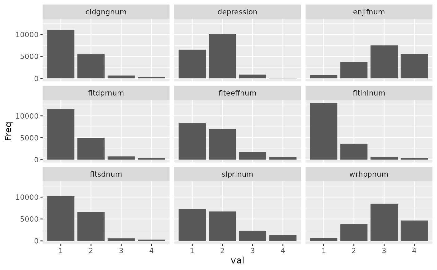
#> Descriptives for healthy_eating scale:
#> Mean: 4.931  SD: 1.131
#> Cronbach's alpha: .66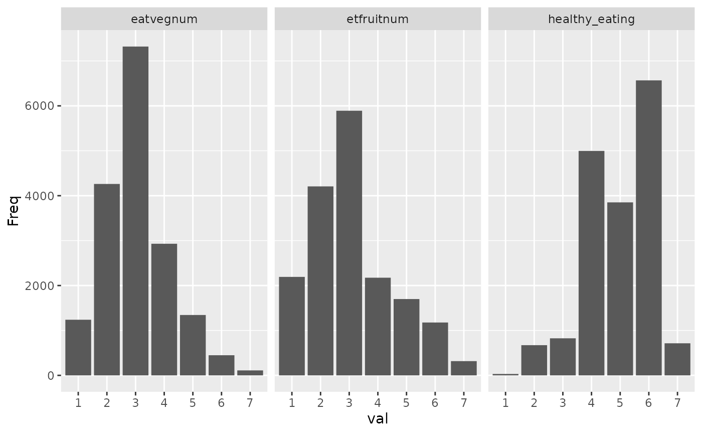
Report correlations
You can use svy_cor_matrix() to calculate weighted
correlations, and then use report_cor_table() to present
them nicely.
ess_survey %>%
  select(agea, health, depression, healthy_eating) %>%
  svy_cor_matrix() %>%
report_cor_table()| Variable | M (SD) | 1 | 2 | 3 |
|---|---|---|---|---|
|
47.87 (18.98) | |
|
|
|
2.23 (0.91) | .30 *** [0.28, 0.32] |
|
|
|
1.66 (0.48) | .05 *** [0.02, 0.07] |
.41 *** [0.39, 0.44] |
|
|
4.93 (1.13) | .17 *** [0.15, 0.19] |
-.09 *** [-0.11, -0.07] |
-.11 *** [-0.13, -0.08] |
| M and SD are used to represent mean and standard deviation, respectively. | ||||
| Values in square brackets indicate the confidence interval for each correlation. | ||||
| † p < .1, * p < .05, ** p < .01, *** p < .001 | ||||
It is often helpful to use different variable names for display. For
this, functions in the package typically accept rename tibbles that
contain an old and a new column. By using the
tibble::tribble notation, they can be entered more cleanly
than named character vectors, and the get_rename_tribble()
helper function creates most of the code.
# Call
# get_rename_tribbles(ess_health, agea, health, depression, healthy_eating, which = "vars")
# to get most of this code

var_renames <- tibble::tribble(
  ~old,             ~new,
   "agea",           "Age",
   "health",         "Poor health",
   "depression",     "Depression",
   "healthy_eating",  "Healthy eating"
)

# If var_names are provided, only variables included in that argument
# are included in the correlation table
ess_survey %>% svy_cor_matrix(var_names = var_renames) %>%
report_cor_table()| Variable | M (SD) | 1 | 2 | 3 |
|---|---|---|---|---|
|
47.87 (18.98) | |
|
|
|
2.23 (0.91) | .30 *** [0.28, 0.32] |
|
|
|
1.66 (0.48) | .05 ** [0.02, 0.07] |
.41 *** [0.39, 0.44] |
|
|
4.93 (1.13) | .17 *** [0.15, 0.19] |
-.09 *** [-0.11, -0.07] |
-.11 *** [-0.13, -0.08] |
| M and SD are used to represent mean and standard deviation, respectively. | ||||
| Values in square brackets indicate the confidence interval for each correlation. | ||||
| † p < .1, * p < .05, ** p < .01, *** p < .001 | ||||
Adding distribution plots
You can add distribution plots to correlation tables for survey data.
These distributions are properly weighted using svyhist()
for discrete variables and svysmooth() for continuous
variables, ensuring they reflect the population rather than just the
sample composition.
ess_survey %>% svy_cor_matrix(var_names = var_renames) %>%
report_cor_table(add_distributions = TRUE, data = ess_survey)| Variable | M (SD) | Distributions | 1 | 2 | 3 |
|---|---|---|---|---|---|
|
47.87 (18.98) |  |
|
|
|
|
2.23 (0.91) |  |
.30 *** [0.28, 0.32] |
|
|
|
1.66 (0.48) |  |
.05 *** [0.02, 0.07] |
.41 *** [0.39, 0.44] |
|
|
4.93 (1.13) |  |
.17 *** [0.15, 0.19] |
-.09 *** [-0.11, -0.06] |
-.11 *** [-0.13, -0.08] |
| M and SD are used to represent mean and standard deviation, respectively. | |||||
| Values in square brackets indicate the confidence interval for each correlation. | |||||
| † p < .1, * p < .05, ** p < .01, *** p < .001 | |||||
The plot_distributions() function can also be used
directly with survey data:
plot_distributions(ess_survey, var_names = var_renames)
#> $Age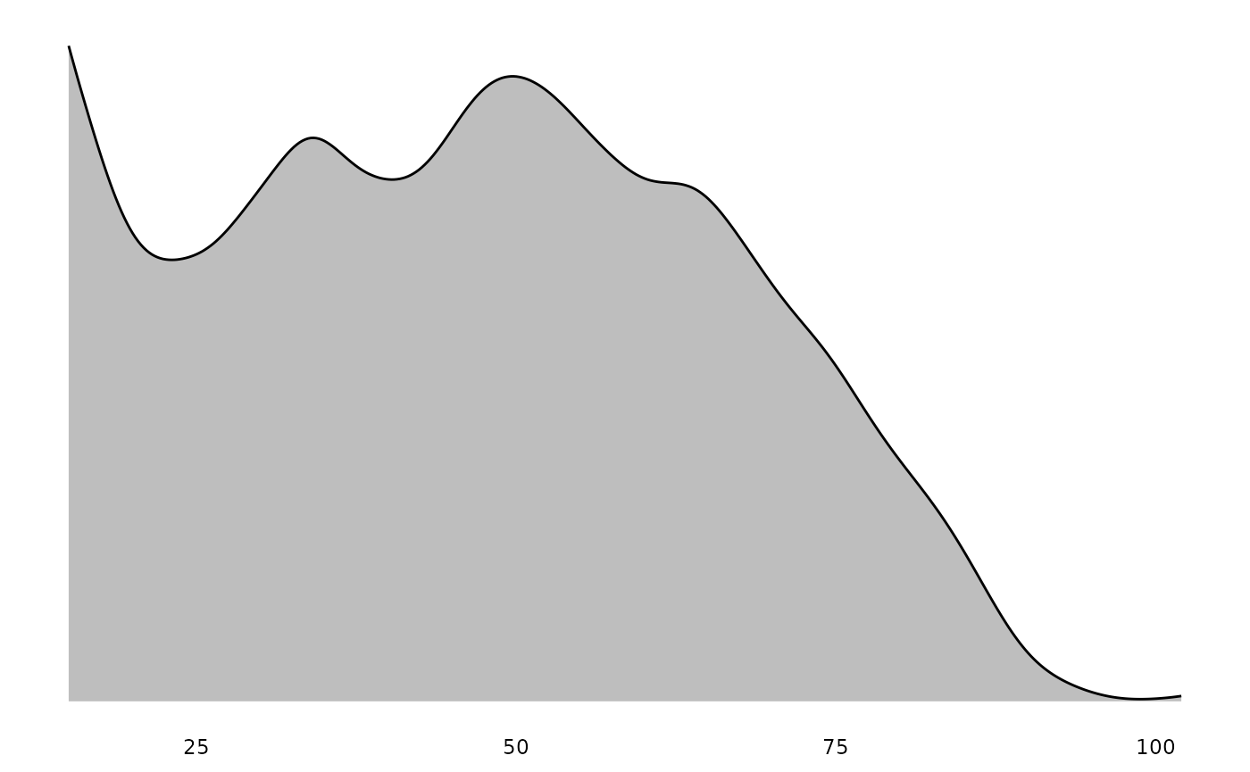
#>
#> $`Poor health`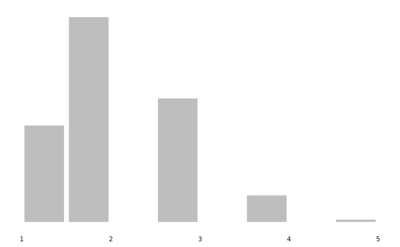
#>
#> $Depression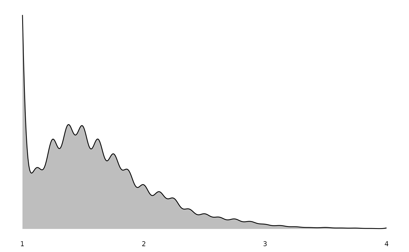
#>
#> $`Healthy eating`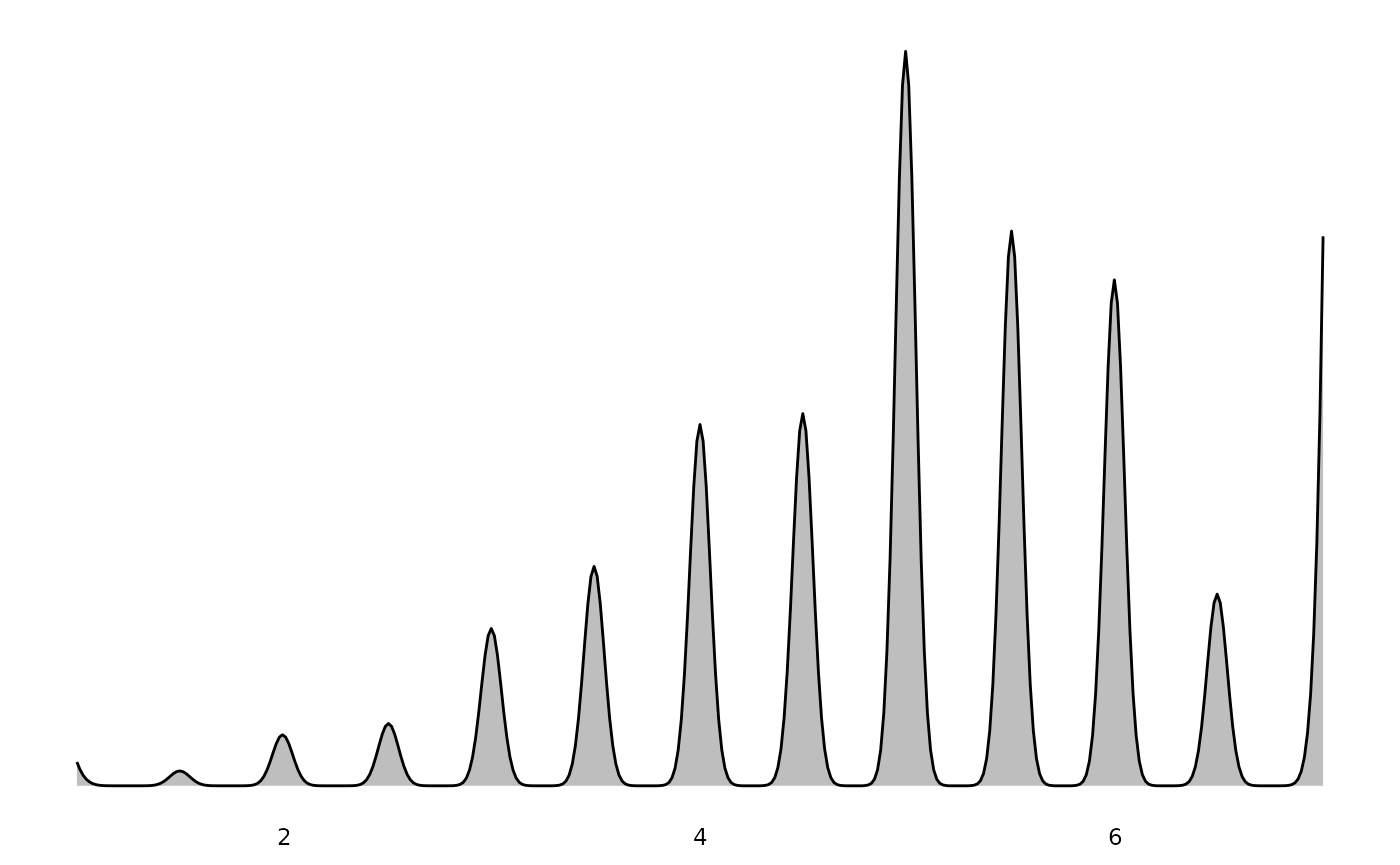
These plots properly account for survey weights, so the distributions shown represent population estimates rather than raw sample frequencies.
Testing significance of difference between two groups
Running a t-test on survey data is easy with
survey::svyttest(). However, getting Cohen’s d as
a measure of effect size, or subsetting to compare just two levels if
there are more in the data is less trivial, and is where
svy_cohen_d_pair() comes in.
# Returns Cohen's d in the 'd' column
svy_cohen_d_pair(ess_survey, "health", "gndr")
#> # A tibble: 1 × 8
#>   pair       d      t    df p.value mean_diff mean_diff_ci.low mean_diff_ci.high
#>   <chr>  <dbl>  <dbl> <dbl>   <dbl>     <dbl>            <dbl>             <dbl>
#> 1 1 & 2 -0.133 -0.120  7217 1.40e-6    -0.120          -0.0714            -0.169
svy_cohen_d_pair(ess_survey, "health", "cntry", pair = c("DE", "GB"))
#> # A tibble: 1 × 8
#>   pair       d     t    df  p.value mean_diff mean_diff_ci.low mean_diff_ci.high
#>   <chr>  <dbl> <dbl> <dbl>    <dbl>     <dbl>            <dbl>             <dbl>
#> 1 DE & … 0.324 0.295  5301 7.94e-25     0.295            0.351             0.239
Running pairwise t-tests
svy_pairwise_t_test() allows to run pairwise t-tests,
e.g., as post-hoc comparisons, between multiple groups in the survey.
p-values are adjusted for multiple comparisons, by default
using the Holm-Bonferroni method.
svy_pairwise_t_test(ess_survey, "health", "cntry", cats = c("DE", "GB", "FR"))
#> # A tibble: 3 × 8
#>   pair          d       t    df  p.value mean_diff mean_diff_ci.low
#>   <chr>     <dbl>   <dbl> <dbl>    <dbl>     <dbl>            <dbl>
#> 1 DE & GB  0.324   0.295   5301 2.38e-24    0.295             0.351
#> 2 DE & FR  0.0956  0.0849  4954 5.88e- 3    0.0849            0.145
#> 3 GB & FR -0.233  -0.210   4177 3.16e-10   -0.210            -0.146
#> # ℹ 1 more variable: mean_diff_ci.high <dbl>