This vignette introduces some of the basic functions that quickly get
you from a dataset to publication-ready outputs. It uses
tidyverse/dplyr-functions alongside
timesaveR as that is the recommended workflow.
Create scales
Let’s create scales for health behaviours and depressive symptoms, each including some reverse coding. For that, scale items need to be included into a list of named character vectors; if any items are to be reversed, they should be added into another list of character vectors.
scales_items <- list(
depression = c("fltdpr", "flteeff", "slprl", "wrhpp", "fltlnl",
"enjlf", "fltsd", "cldgng"),
healthy_eating = c("etfruit", "eatveg")
)
scales_reverse <- list(
depression = c("wrhpp", "enjlf"),
healthy_eating = c("etfruit", "eatveg")
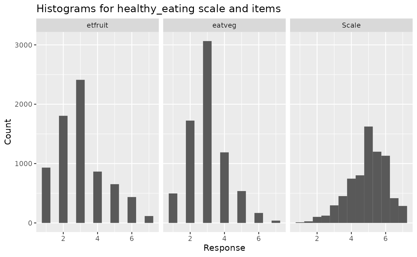
)Then, the make_scales() command can be used to
calculate scale scores as well as descriptives. By
default, it also returns histograms showing the distribution of each
item and the resulting scale, which can help to spot problems. By
default, it also returns both scale scores and
descriptives that can be processed separately.
scales <- make_scales(ess_health, items = scales_items, reversed = scales_reverse)
#> The following scales will be calculated with specified reverse coding:
#> depression, healthy_eating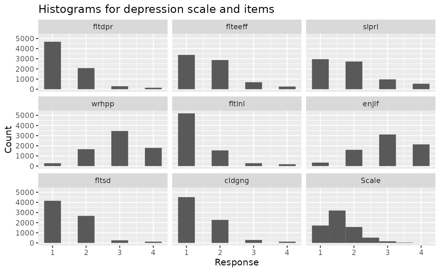
#Check descriptives, including reliability
scales$descriptives %>% round_df()
#> # A tibble: 2 × 10
#>   Scale      n_items reliability reliability_method  mean    SD reversed rev_min
#>   <chr>        <dbl>       <dbl> <chr>              <dbl> <dbl> <chr>      <dbl>
#> 1 depression       8        0.8  cronbachs_alpha     1.67  0.48 wrhpp e…       1
#> 2 healthy_e…       2        0.66 spearman_brown      4.97  1.11 etfruit…       1
#> # ℹ 2 more variables: rev_max <dbl>, text <chr>

#Add scale scores to dataset
ess_health <- cbind(ess_health, scales$scores)
Report correlations and descriptive statistics
At the start of a data analysis project, we are often interested in
descriptive statistics, variable distributions and correlations. As far
as numerical variables are concerned, all of them can be reported in a
pretty table with the report_cor_table() function. That
function needs a correlation matrix as its first argument, which can
usually be created with the cor_matrix() function.
ess_health %>%
  select(agea, health, depression, healthy_eating) %>%
  cor_matrix() %>%
report_cor_table()| Variable | M (SD) | 1 | 2 | 3 |
|---|---|---|---|---|
|
50.61 (18.51) | |
|
|
|
2.26 (0.92) | .28 *** [0.25, 0.30] |
|
|
|
1.67 (0.48) | .03 * [0.00, 0.05] |
.42 *** [0.40, 0.44] |
|
|
4.97 (1.11) | .17 *** [0.15, 0.19] |
-.09 *** [-0.11, -0.07] |
-.13 *** [-0.15, -0.10] |
| M and SD are used to represent mean and standard deviation, respectively. | ||||
| Values in square brackets indicate the confidence interval for each correlation. | ||||
| † p < .1, * p < .05, ** p < .01, *** p < .001 | ||||
It is often helpful to use different variable names for display. For
this, functions in the package typically accept rename tibbles that
contain an old and a new column. By using the
tibble::tribble notation, they can be entered more cleanly
that named character vectors, and the get_rename_tribble()
helper function creates most of the code.
# Use get_rename_tribbles to get most of this code
var_renames <- tibble::tribble(
  ~old,             ~new,
   "agea",           "Age",
   "health",         "Poor health",
   "depression",     "Depression",
   "healthy_eating",  "Healthy eating"
)

# If var_names are provided, only variables included in that argument
# are included in the correlation table
ess_health %>% cor_matrix(var_names = var_renames) %>% report_cor_table()| Variable | M (SD) | 1 | 2 | 3 |
|---|---|---|---|---|
|
50.61 (18.51) | |
|
|
|
2.26 (0.92) | .28 *** [0.25, 0.30] |
|
|
|
1.67 (0.48) | .03 * [0.00, 0.05] |
.42 *** [0.40, 0.44] |
|
|
4.97 (1.11) | .17 *** [0.15, 0.19] |
-.09 *** [-0.11, -0.07] |
-.13 *** [-0.15, -0.10] |
| M and SD are used to represent mean and standard deviation, respectively. | ||||
| Values in square brackets indicate the confidence interval for each correlation. | ||||
| † p < .1, * p < .05, ** p < .01, *** p < .001 | ||||
Often, it is interesting to also include variable
distributions into this initial data summary table. This can
also be done with the report_cor_table() function. By
default, variables with 5 distinct values or fewer are shown with a
histogram, while for those with more values, a density plot is provided
- but this can be changed with the plot_type argument.
ess_health %>% cor_matrix(var_names = var_renames) %>%
report_cor_table(add_distributions = TRUE, data = ess_health)| Variable | M (SD) | Distributions | 1 | 2 | 3 |
|---|---|---|---|---|---|
|
50.61 (18.51) |  |
|
|
|
|
2.26 (0.92) |  |
.28 *** [0.25, 0.30] |
|
|
|
1.67 (0.48) |  |
.03 * [0.00, 0.05] |
.42 *** [0.40, 0.44] |
|
|
4.97 (1.11) |  |
.17 *** [0.15, 0.19] |
-.09 *** [-0.11, -0.07] |
-.13 *** [-0.15, -0.10] |
| M and SD are used to represent mean and standard deviation, respectively. | |||||
| Values in square brackets indicate the confidence interval for each correlation. | |||||
| † p < .1, * p < .05, ** p < .01, *** p < .001 | |||||
Describe categorical variables and their relation with an outcome
Often, we are also interested in how the means of an outcome variable differ between different groups. It can be fiddly to get these tables and the pairwise significance tests done, but this function does it in a breeze.
If you want to rename variable levels as well as names, the
get_rename_tribbles() function becomes a real
timesaver.
# Start with get_rename_tribbles(ess_health, gndr, cntry) in the console

var_renames <- tibble::tribble(
    ~old,     ~new,
    "gndr",   "Gender",
    "cntry",  "Country"
)

level_renames <- tibble::tribble(
    ~var,     ~level_old, ~level_new,
    "gndr",   "1",        "male",
    "gndr",   "2",        "female",
    "cntry",  "DE",       "Germany",
    "cntry",  "FR",       "France",
    "cntry",  "GB",       "UK"
)
Then run report_cat_vars() to get a table with the
distribution of the categories and their association with the outcome
variable.
report_cat_vars(ess_health, health, gndr, cntry, var_names = var_renames,
level_names = level_renames)| N | Share | M (SD) | |
|---|---|---|---|
| Gender | |||
| male | 3482 | 48.2% | 2.23 (0.90) b |
| female | 3744 | 51.8% | 2.30 (0.93) a |
| Country | |||
| Germany | 3045 | 42.1% | 2.34 (0.88) a |
| France | 1917 | 26.5% | 2.29 (0.89) a |
| UK | 2264 | 31.3% | 2.14 (0.97) b |
|
M and SD are used to
represent mean and standard deviation for health for that group,
respectively. |
|||
|
Within each variable, the means of groups with
different superscripts differ with p < .05 (p-values were adjusted using the Holm-method.) |
|||
Report regression models with standardized coefficients
In psychology, it is often expected that regression models are
reported with both unstandardised (B) and standardized (β) coefficients.
This can be fiddly and lead to redundant information. The
lm_std() function easily runs linear regression models that
return standardised coefficients and the
report_lm_with_std() function creates side-by-side
regression tables that minimize redundancy.
At the most basic, you just need to run two models and pass them to the reporting function:
ess_health$gndr <- factor(ess_health$gndr)

#Standard lm model
mod1 <- lm(depression ~ agea + gndr + health + cntry, ess_health)

#Model with standardised coefficients
mod2 <- lm_std(depression ~ agea + gndr + health + cntry, ess_health)

report_lm_with_std(mod1, mod2)
#> Warning: The `tidy()` method for objects of class `lm_std` is not maintained by the broom team, and is only supported through the `lm` tidier method. Please be cautious in interpreting and reporting broom output.
#>
#> This warning is displayed once per session.|
|
|
|
|---|---|---|
| (Intercept) | 1.20 (0.02)*** | -0.14 [-0.18, -0.10] |
| agea | -0.00 (0.00)*** | -0.10 [-0.12, -0.08] |
| gndr2 | 0.12 (0.01)*** | 0.24 [0.20, 0.28] |
| health | 0.23 (0.01)*** | 0.44 [0.42, 0.47] |
| cntryFR | -0.01 (0.01) | -0.02 [-0.08, 0.03] |
| cntryGB | 0.04 (0.01)** | 0.08 [0.03, 0.13] |
| N | 7171 | |
| R2 | .20 | |
| F-tests |
F(5, 7165) = 358.25, p < .001 |
|
| † p < .1, * p < .05, ** p < .01, *** p < .001 | ||
Often, the coefficient names - particularly for dummy variables - are
not particularly clear or pleasing. In such cases, they can be renamed
easily - again, there is a helper function
(get_coef_rename_tribble()) that creates most of the
necessary code. In the new names, you can use markdown formatting, for
instance to add information on reference levels.
# get_coef_rename_tribble(mod1) is the starting point.

coef_names <- tibble::tribble(
  ~old,           ~new,
   "(Intercept)",  "*(Intercept)*",
   "agea",         "Age",
   "gndr2",        "Gender *(female)*",
   "health",       "Poor health",
   "cntryFR",      "France *(vs DE)*",
   "cntryGB",      "UK *(vs DE)*"
)

report_lm_with_std(mod1, mod2, coef_renames = coef_names)|
|
|
|
|---|---|---|
| (Intercept) | 1.20 (0.02)*** | -0.14 [-0.18, -0.10] |
| Age | -0.00 (0.00)*** | -0.10 [-0.12, -0.08] |
| Gender (female) | 0.12 (0.01)*** | 0.24 [0.20, 0.28] |
| Poor health | 0.23 (0.01)*** | 0.44 [0.42, 0.47] |
| France (vs DE) | -0.01 (0.01) | -0.02 [-0.08, 0.03] |
| UK (vs DE) | 0.04 (0.01)** | 0.08 [0.03, 0.13] |
| N | 7171 | |
| R2 | .20 | |
| F-tests |
F(5, 7165) = 358.25, p < .001 |
|
| † p < .1, * p < .05, ** p < .01, *** p < .001 | ||
You can also display two nested models side-by-side and get the F-change significance test. (More models can be displayed, but not yet statistically tested against each other.) To enable model comparisons, all models need to be fitted on the same dataset, so that I will first omit missing data.
ess_health <- tidyr::drop_na(ess_health)

mod1 <- lm(depression ~ agea + gndr + health + cntry, ess_health)
mod2 <- lm_std(depression ~ agea + gndr + health + cntry, ess_health)


mod3 <- lm(depression ~ agea * gndr + eisced + health + cntry, ess_health)
mod4 <- lm_std(depression ~ agea * gndr + eisced + health + cntry, ess_health)

coef_names <- tibble::tribble(
  ~old,           ~new,
   "(Intercept)",  "*(Intercept)*",
   "agea",         "Age",
   "gndr2",        "Gender *(female)*",
   "health",       "Poor health",
   "cntryFR",      "France *(vs DE)*",
   "cntryGB",      "UK *(vs DE)*",
   "eisced",       "Education",
   "agea:gndr2",   "Age x Female",
)

report_lm_with_std(mod = list(mod1, mod3), mod_std = list(mod2, mod4),
                   coef_renames = coef_names, R2_change = TRUE,
                   model_names = c("Base model", "Extended model"))
#> Warning: Automatic coercion from double to character was deprecated in purrr 1.0.0.
#> ℹ Please use an explicit call to `as.character()` within `map_chr()` instead.
#> ℹ The deprecated feature was likely used in the timesaveR package.
#>   Please report the issue at
#>   <https://github.com/LukasWallrich/timesaveR/issues>.
#> This warning is displayed once every 8 hours.
#> Call `lifecycle::last_lifecycle_warnings()` to see where this warning was
#> generated.|
Base model
|
Extended model
|
|||
|---|---|---|---|---|
|
|
|
|
|
|
| (Intercept) | 1.21 (0.02)*** | -0.14 [-0.18, -0.10] | 1.27 (0.02)*** | -0.14 [-0.18, -0.10] |
| Age | -0.00 (0.00)*** | -0.10 [-0.12, -0.08] | -0.00 (0.00)*** | -0.14 [-0.17, -0.10] |
| Gender (female) | 0.11 (0.01)*** | 0.24 [0.20, 0.28] | 0.03 (0.03) | 0.24 [0.20, 0.28] |
| Poor health | 0.23 (0.01)*** | 0.44 [0.42, 0.46] | 0.23 (0.01)*** | 0.44 [0.42, 0.46] |
| France (vs DE) | -0.01 (0.01) | -0.03 [-0.08, 0.02] | -0.01 (0.01) | -0.03 [-0.08, 0.02] |
| UK (vs DE) | 0.04 (0.01)** | 0.08 [0.03, 0.13] | 0.04 (0.01)** | 0.08 [0.03, 0.13] |
| Education | -0.00 (0.00)† | -0.02 [-0.04, 0.00] | ||
| Age x Female | 0.00 (0.00)** | 0.07 [0.02, 0.11] | ||
| N | 6852 | 6852 | ||
| R2 | .20 | .20 | ||
| F-tests |
F(5, 6846) = 337.06, p < .001 |
F(7, 6844) = 243.10, p < .001 |
||
| Change | ΔR2 = .00, F(2, 6844) = 6.78, p = .001 | |||
| † p < .1, * p < .05, ** p < .01, *** p < .001 | ||||
Happy exploring, and please do report bugs and unexpected behaviors by opening an issue on GitHub or emailing me on lukas.wallrich@gmail.com